Python #1 CNN

책을 읽으면서 정리한 내용

• 그냥 임의대로 본인 기준대로 정리한 내용이니 빠진 부분에 대해서는 책을 직접보면 훨씬 더 잘 정리되어 있음.

Image to column

def im2col(input_data, filter_h, filter_w, stride=1, pad=0):
 """다수의 이미지를 입력받아 2차원 배열로 변환한다(평탄화).

Parameters
 ----------
 input_data : 4차원 배열 형태의 입력 데이터(이미지 수, 채널 수, 높이, 너비)
 filter_h : 필터의 높이
 filter_w : 필터의 너비
 stride : 스트라이드
 pad : 패딩

Returns
 -------
 col : 2차원 배열
 """
 N, C, H, W = input_data.shape
                  # 입력 데이터의 정보를 얻는다.
                  # number of data set
                  # number of channel
                  # Height
                  # Width
 out_h = (H + 2*pad - filter_h)//stride + 1
                  # // 은 몫 연산자임... 
 out_w = (W + 2*pad - filter_w)//stride + 1

img = np.pad(input_data, 
             [(0,0), (0,0), (pad, pad), (pad, pad)], 
             'constant')
 col = np.zeros((N, C, filter_h, filter_w, out_h, out_w))

for y in range(filter_h):
     y_max = y + stride*out_h
     for x in range(filter_w):
         x_max = x + stride*out_w
          col[:, :, y, x, :, :] = 
                img[:, :, y:y_max:stride, x:x_max:stride]

col = col.transpose(0, 4, 5, 1, 2, 3).reshape(N*out_h*out_w, -1)
return col

위의 함수에서  np.pad를 테스트 해 보기 위해서 아래와 같이 함수를 만들어서 테스트 해보면,

import numpy as np # Import Numphy
x = np.random.rand(1,1,3,3) # Generate Random
              # Width 3
              # Height 3
              # channel 1
              # Data set 1

print (x.shape)
print (" Random data set" )
print ( x[0,0] )

pad = 1

print ("Pad = " , pad )

img = np.pad(x ,  
             [ (0,0) , (0,0) , (pad,pad) , (pad,pad) ] , 
            'constant')

print ( "Img's shape = " , img.shape )
print ( img[0,0] )

실행 결과는 아래와 같이 나온다.

MacBook-Pro:Chap7 freegear$ python padtest.py
(1, 1, 3, 3)
 Random data set
[[ 0.55114585 0.78247964 0.09729986]
 [ 0.87498808 0.35761342 0.41334762]
 [ 0.20798783 0.29943406 0.14252441]]
Pad = 1
Img's shape = (2, 1, 5, 5)
[[ 0. 0. 0. 0. 0. ]
 [ 0. 0.55114585 0.78247964 0.09729986 0. ]
 [ 0. 0.87498808 0.35761342 0.41334762 0. ]
 [ 0. 0.20798783 0.29943406 0.14252441 0. ]
 [ 0. 0. 0. 0. 0. ]]

pad 만큼 붙어서 나온다.

pad 함수의 인자는 아래와 같다.

array : array_like of rank N

Input array

pad_width : {sequence, array_like, int}

Number of values padded to the edges of each axis.

((before_1, after_1), … (before_N, after_N))

unique pad widths for each axis. ((before, after),) yields same before and after pad for each axis. (pad,) or int is a shortcut for before = after = pad width for all axes.

mode : str or function

각 축에 해당하는 것을 붙인다. 앞서의 예에서 실제 함수는

img = np.pad(x , 
     [ (0,0) , (0,0) , (1,1) , (1,1) ] , 
 'constant')

이 된다.

여기서 첫째 인자는  dataset 에 붙이는 pad가 0 즉 없다이고

두번째 인자는” channel 역시 pad가 없다.”

세번째 인자인 (1,1)은 데이터 세트 중에서 가로와 세로측 시작 위치에 붙이는 pad의 숫자를 의미한다.

img = np.pad(x , 
       [ (0,0) , (0,0) , (pad,pad + 1) , (pad + 1 ,pad) ] , 
       'constant')

테스트를 위해서 위와 같이 수정해서 생성하면 아래와 같은 결과가 나온다.

MacBook-Pro:Chap7 freegear$ python padtest.py
(1, 1, 3, 3)
 Random data set
[[ 0.26100326 0.59634124 0.26162682]
 [ 0.34669303 0.17809826 0.43675991]
 [ 0.28356393 0.91815353 0.17761533]]
Pad = 1
Img's shape = (1, 1, 6, 6)
[[ 0. 0. 0. 0. 0. 0. ]
 [ 0. 0. 0.26100326 0.59634124 0.26162682 0. ]
 [ 0. 0. 0.34669303 0.17809826 0.43675991 0. ]
 [ 0. 0. 0.28356393 0.91815353 0.17761533 0. ]
 [ 0. 0. 0. 0. 0. 0. ]
 [ 0. 0. 0. 0. 0. 0. ]]

(pad,pad + 1)

세로축으로 시작할때 pad 1을 끝날 때 pad 2를 추가하는 것을 의미한다.

따라서 세로축으로 3이 늘어나지만, 앞 부분은 1을 뒷 부분은 2칸 늘린 형태가 된다.

(pad + 1 ,pad)

가로 축으로 시작할 때 pad를 2로 끝날 때 Pad를 1로 추가한다.

col = np.zeros((N, C, filter_h, filter_w, out_h, out_w))

영행렬을 만들어 준다. 인자는 다음과 같다.

numpy.zeros(shape, dtype=float, order=’C’)

Return a new array of given shape and type, filled with zeros.

실제 변환은 아래와 같다.

for y in range(filter_h):
    y_max = y + stride*out_h
    for x in range(filter_w):
       x_max = x + stride*out_w
       col[:, :, y, x, :, :] = 
          img[:, :, y:y_max:stride, x:x_max:stride]

필터의 크기에 맞게 y를 선택한다.  stride 만큼 넓은 면적을 만들어가면서 최대 값을 만든다.

마찬가지로 x값도 필터의 넓이 값을 기준으로 만들고 stride와 출력을 고려하여서 최대 값을 만든다. 그리고 데이터를 이미지에서 오려 낸다.

이미지 내에서 시작 위치는 y 이고, 최댓값만큼 크기를 잡고, x도 마찬가지로 잡아서 해당 위치의 값들을 col로 옮긴다.

col = col.transpose(0, 4, 5, 1, 2, 3).reshape(N*out_h*out_w, -1)

이렇게 보면 명확하게 들어오지 않기 때문에 테스트를 위해서 별도로 함수를 넣어서 테스트 해 본다.

import sys, os
import numpy as np

sys.path.append(os.pardir)
from common.util import im2col

x1 = np.random.rand(1,1,5,5)
      # Data Set
      # Num of channel
      # Height
      # Width



col1 = im2col(x1,3,3,stride=1,pad = 0 )
print(col1.shape)
print(x1)
print(col1)

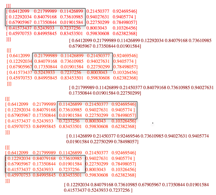
위와같이  5×5  데이터를 만들어서 여기에 3×3 필터를 연산하기 위한 im2col을 걸어본다.

그 결과는 아래와 같다

MacBook-Pro:Chap7 freegear$ python im2col_test.py
(9, 9)
[[[[ 0.6412099 0.21799989 0.11426899 0.21450377 0.92469546]
 [ 0.12292034 0.84079168 0.73610985 0.94027631 0.9405774 ]
 [ 0.67905967 0.17350844 0.01901584 0.22750299 0.78498057]
 [ 0.41573437 0.5243933 0.7237256 0.8003043 0.10326456]
 [ 0.45970753 0.84995845 0.83453501 0.59830608 0.62382368]]]]
[[ 0.6412099 0.21799989 0.11426899 0.12292034 0.84079168 0.73610985
 0.67905967 0.17350844 0.01901584]
 [ 0.21799989 0.11426899 0.21450377 0.84079168 0.73610985 0.94027631
 0.17350844 0.01901584 0.22750299]
 [ 0.11426899 0.21450377 0.92469546 0.73610985 0.94027631 0.9405774
 0.01901584 0.22750299 0.78498057]
 [ 0.12292034 0.84079168 0.73610985 0.67905967 0.17350844 0.01901584
 0.41573437 0.5243933 0.7237256 ]
 [ 0.84079168 0.73610985 0.94027631 0.17350844 0.01901584 0.22750299
 0.5243933 0.7237256 0.8003043 ]
 [ 0.73610985 0.94027631 0.9405774 0.01901584 0.22750299 0.78498057
 0.7237256 0.8003043 0.10326456]
 [ 0.67905967 0.17350844 0.01901584 0.41573437 0.5243933 0.7237256
 0.45970753 0.84995845 0.83453501]
 [ 0.17350844 0.01901584 0.22750299 0.5243933 0.7237256 0.8003043
 0.84995845 0.83453501 0.59830608]
 [ 0.01901584 0.22750299 0.78498057 0.7237256 0.8003043 0.10326456
 0.83453501 0.59830608 0.62382368]]
(90, 75)

처음 프린트 된것이 5×5  데이터 행렬이다.

두번째 프린트 한것이 3×3 필터를 넣기 위한 im2col의 결과이다.

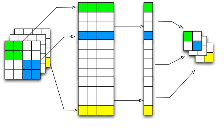
이해를 위해서 그림으로 다시 그려보면 아래와 같은 형태의 그림이 나온다.

….

위와 같이 3×3을 위한 매트릭스를 1차원 배열로 만들어 준다.

def col2im(col, input_shape, filter_h, filter_w, stride=1, pad=0):
 """(im2col과 반대) 2차원 배열을 입력받아 다수의 이미지 묶음으로 변환한다.

Parameters
 ----------
 col : 2차원 배열(입력 데이터)
 input_shape : 원래 이미지 데이터의 형상（예：(10, 1, 28, 28)）
 filter_h : 필터의 높이
 filter_w : 필터의 너비
 stride : 스트라이드
 pad : 패딩

Returns
 -------
 img : 변환된 이미지들
 """

 N, C, H, W = input_shape
 out_h = (H + 2*pad - filter_h)//stride + 1
 out_w = (W + 2*pad - filter_w)//stride + 1
 col = col.reshape(
      N, 
      out_h, out_w, 
      C, 
      filter_h, filter_w).transpose(0, 3, 4, 5, 1, 2)

      img = np.zeros(
               (N, C, 
               H + 2*pad + stride - 1, W + 2*pad + stride - 1)
            )

 for y in range(filter_h):
      y_max = y + stride*out_h
      for x in range(filter_w):
           x_max = x + stride*out_w
           img[:, :, y:y_max:stride, x:x_max:stride] += 
                col[:, :, y, x, :, :]

return img[:, :, pad:H + pad, pad:W + pad]

이제 이 함수를 이용해서 convolution을 구현한다.

# Convolution
import numpy as np

class Convolution
 def __iit__(self, W b , stride = 1 , pad = 0 ):
 self.W = W
 self.b = b
 self.stride = stride
 self.pad = pad

def forward(self,x):
 FN, C, FH , FW = self.W.shape
 # FN : number of Filter
 # C  : Channel
 # FH : Height of Filter
 # FW : Width of Filter

 N,C,H,W = x.shape
 out_h = int(1+(H+2*self.pad - FH)/self.stride)
 out_w = int(1+(W+2*self.pad - FW)/self.stride)

col = im2col(x, FH , FW , self.stride , self.pad)
col_W = self.W.reshape(FN,-1).T
out = np.dot(col, col_W) + self.b

out = out.reshape(N, out_h , out_w , -1 ).transpose(0,3,1,2)

return out

CNN

class Pooling:
 def __init__(self, pool_h, pool_w, stride=1, pad=0):
 self.pool_h = pool_h
 self.pool_w = pool_w
 self.stride = stride
 self.pad = pad

self.x = None
 self.arg_max = None

def forward(self, x):
 N, C, H, W = x.shape
 out_h = int(1 + (H - self.pool_h) / self.stride)
 out_w = int(1 + (W - self.pool_w) / self.stride)

col = im2col(
             x, 
             self.pool_h, 
             self.pool_w, 
             self.stride, self.pad)

 col = col.reshape(-1, self.pool_h*self.pool_w)
 arg_max = np.argmax(col, axis=1)
 out = np.max(col, axis=1)
 out = out.reshape(N, out_h, out_w, C).transpose(0, 3, 1, 2)

 self.x = x
 self.arg_max = arg_max

return out

def backward(self, dout):
 dout = dout.transpose(0, 2, 3, 1)

pool_size = self.pool_h * self.pool_w
 dmax = np.zeros((dout.size, pool_size))
 dmax[np.arange(self.arg_max.size), self.arg_max.flatten()] = 
        dout.flatten()
 dmax = dmax.reshape(dout.shape + (pool_size,))

dcol = dmax.reshape(
               dmax.shape[0] * dmax.shape[1] * dmax.shape[2], 
               -1)
 dx = col2im(dcol, 
             self.x.shape, 
             self.pool_h, self.pool_w, 
             self.stride, self.pad)

return dx

아래는 pooling의 진행 flow chart 입니다.

위와 같이 이미지를 풀어서 연산하고 다시 이미지를 합친다.

이러한 과정으로 연산하는 것이 이미지 자체를 2d로 하여서 연산하는 것에 비해서 빠르다는 것이 의견이다.

Simple CNN

다음과 같이 구성된다.

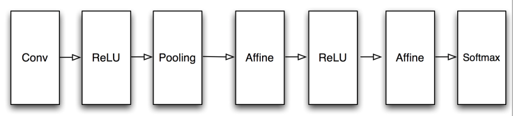
SimpleConvNet으로 구현한다.

class SimpleConvNet:
 """단순한 합성곱 신경망

conv - relu - pool - affine - relu - affine - softmax

Parameters
 ----------
 input_size : 입력 크기（MNIST의 경우엔 784）
 hidden_size_list : 각 은닉층의 뉴런 수를 담은 리스트（e.g. [100, 100, 100]）
 output_size : 출력 크기（MNIST의 경우엔 10）
 activation : 활성화 함수 - 'relu' 혹은 'sigmoid'
 weight_init_std : 가중치의 표준편차 지정（e.g. 0.01）
 'relu'나 'he'로 지정하면 'He 초깃값'으로 설정
 'sigmoid'나 'xavier'로 지정하면 'Xavier 초깃값'으로 설정
 """
 def __init__(self, 
              input_dim=(1, 28, 28), # 입력 데이터의 차원, 
              conv_param={'filter_num':30, # 필터의 수
                          'filter_size':5, # 필터의 크기
                          'pad':0, 'stride':1},
              hidden_size=100, # 은닉층의 뉴런 수...
              output_size=10,  # 츨력층의 뉴런 수...
              weight_init_std=0.01):# 초기화의 가중치 초기 편차

 # 데이터 꺼내기
 filter_num = conv_param['filter_num']  
 filter_size = conv_param['filter_size']
 filter_pad = conv_param['pad']
 filter_stride = conv_param['stride']

 # Input Size
 input_size = input_dim[1]

 conv_output_size = (input_size - filter_size + 2*filter_pad) / filter_stride + 1
 pool_output_size = int(filter_num * (conv_output_size/2) * (conv_output_size/2))

 # 가중치 초기화
 self.params = {}
 self.params['W1'] = weight_init_std * \
                        np.random.randn(
                                filter_num, input_dim[0], 
                                filter_size, filter_size)
 self.params['b1'] = np.zeros(filter_num)
 self.params['W2'] = weight_init_std * \
                        np.random.randn(
                          pool_output_size, 
                          hidden_size
                        )
 self.params['b2'] = np.zeros(hidden_size)
 self.params['W3'] = weight_init_std * \
                        np.random.randn(
                            hidden_size, 
                            output_size)
 self.params['b3'] = np.zeros(output_size)
........

def predict(self, x):
    for layer in self.layers.values():
        x = layer.forward(x)

    return x

def loss(self, x, t):
"""손실 함수를 구한다.

Parameters
----------
x : 입력 데이터
t : 정답 레이블
"""
    y = self.predict(x)
    return self.last_layer.forward(y, t)
...


def gradient(self, x, t):
"""기울기를 구한다(오차역전파법).

Parameters
 ----------
 x : 입력 데이터
 t : 정답 레이블

Returns
 -------
 각 층의 기울기를 담은 사전(dictionary) 변수
 grads['W1']、grads['W2']、... 각 층의 가중치
 grads['b1']、grads['b2']、... 각 층의 편향
 """
# forward
self.loss(x, t)

# backward
dout = 1
dout = self.last_layer.backward(dout)

layers = list(self.layers.values())
layers.reverse()
for layer in layers:
dout = layer.backward(dout)

# 결과 저장
grads = {}
grads['W1'], grads['b1'] = self.layers['Conv1'].dW, self.layers['Conv1'].db
grads['W2'], grads['b2'] = self.layers['Affine1'].dW, self.layers['Affine1'].db
grads['W3'], grads['b3'] = self.layers['Affine2'].dW, self.layers['Affine2'].db

return grads

실행은 아래와 같이 하여서 테스트 해 본다.

코드는 아래와 같다.

train_convnet.py

# coding: utf-8
import sys, os
sys.path.append(os.pardir)  # 부모 디렉터리의 파일을 가져올 수 있도록 설정
import numpy as np
import matplotlib.pyplot as plt
from dataset.mnist import load_mnist
from simple_convnet import SimpleConvNet
from common.trainer import Trainer

# 데이터 읽기
(x_train, t_train), (x_test, t_test) = load_mnist(flatten=False)

max_epochs = 20

network = SimpleConvNet(
                input_dim=(1,28,28),
                conv_param = {
                     'filter_num': 30, 
                     'filter_size': 5, 
                     'pad': 0, 'stride': 1},
                hidden_size=100, 
                output_size=10, 
                weight_init_std=0.01)

 trainer = Trainer(
               network, x_train, t_train, x_test, t_test,
               epochs=max_epochs, mini_batch_size=100,
               optimizer='Adam', optimizer_param={'lr': 0.001},
               evaluate_sample_num_per_epoch=1000)

trainer.train()

# 매개변수 보존
network.save_params("params.pkl")
print("Saved Network Parameters!")

# 그래프 그리기
markers = {'train': 'o', 'test': 's'}
x = np.arange(max_epochs)
plt.plot(x, trainer.train_acc_list, 
                    marker='o', label='train', markevery=2)
plt.plot(x, trainer.test_acc_list, 
                    marker='s', label='test', markevery=2)
plt.xlabel("epochs")
plt.ylabel("accuracy")
plt.ylim(0, 1.0)
plt.legend(loc='lower right')
plt.show()

MacBook-Pro:ch07 freegear$ python train_convnet.py
train loss:2.30039607803
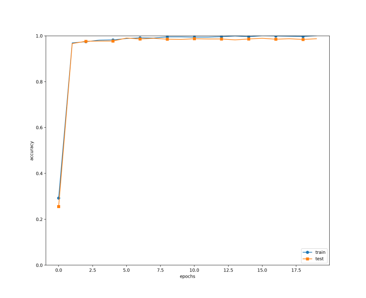
=== epoch:1, train acc:0.293, test acc:0.256 ===
train loss:2.29849717638
train loss:2.29358600789
train loss:2.29119024714
train loss:2.28272736937
train loss:2.27373523644
train loss:2.26121156158
……..

……….
train loss:0.0699663902099
train loss:0.145968228086
train loss:0.0653722496018
=== epoch:2, train acc:0.969, test acc:0.966 ===
train loss:0.0828185561079
train loss:0.220809735512
train loss:0.151240162859

…

train loss:5.91533025357e-05
train loss:0.00175553779364
=============== Final Test Accuracy ===============
test acc:0.9894
Saved Network Parameters!

실행 결과는 아래와 같은 그래프로 나온다.

트레이닝을 위한 class는 아래와 같이 정의 된다.

class Trainer:
 """신경망 훈련을 대신 해주는 클래스
 """
 def __init__(self, network, x_train, t_train, x_test, t_test,
 epochs=20, mini_batch_size=100,
 optimizer='SGD', optimizer_param={'lr':0.01},
 evaluate_sample_num_per_epoch=None, verbose=True):
      self.network = network
     self.verbose = verbose
     self.x_train = x_train
     self.t_train = t_train
     self.x_test = x_test
     self.t_test = t_test
     self.epochs = epochs
     self.batch_size = mini_batch_size
     self.evaluate_sample_num_per_epoch = 
                   evaluate_sample_num_per_epoch

# optimzer
 optimizer_class_dict = {
       'sgd':SGD, 'momentum':Momentum, 'nesterov':Nesterov,
       'adagrad':AdaGrad, 'rmsprpo':RMSprop, 'adam':Adam}
        self.optimizer = 
          optimizer_class_dict[optimizer.lower()](**optimizer_param)

self.train_size = x_train.shape[0]
 self.iter_per_epoch = max(self.train_size / mini_batch_size, 1)
 self.max_iter = int(epochs * self.iter_per_epoch)
 self.current_iter = 0
 self.current_epoch = 0

self.train_loss_list = []
 self.train_acc_list = []
 self.test_acc_list = []

def train_step(self):
 batch_mask = np.random.choice(self.train_size, self.batch_size)
        # Train Size의 데이터 세트에서 
        # Batch Size 만큼의 데이터 세트를 만든다.

 x_batch = self.x_train[batch_mask]
 t_batch = self.t_train[batch_mask]

 grads = self.network.gradient(x_batch, t_batch)
 self.optimizer.update(self.network.params, grads)

 loss = self.network.loss(x_batch, t_batch)
 self.train_loss_list.append(loss)
 if self.verbose: print("train loss:" + str(loss))

 if self.current_iter % self.iter_per_epoch == 0:
     self.current_epoch += 1

 x_train_sample, t_train_sample = self.x_train, self.t_train
 x_test_sample, t_test_sample = self.x_test, self.t_test
 if not self.evaluate_sample_num_per_epoch is None:
     t = self.evaluate_sample_num_per_epoch
     x_train_sample, t_train_sample = 
            self.x_train[:t], self.t_train[:t]
     x_test_sample, t_test_sample = self.x_test[:t], self.t_test[:t]

 train_acc = self.network.accuracy(x_train_sample, t_train_sample)
 test_acc = self.network.accuracy(x_test_sample, t_test_sample)
 self.train_acc_list.append(train_acc)
 self.test_acc_list.append(test_acc)

  if self.verbose: print("=== epoch:" + str(self.current_epoch) + ",
                          train acc:" + str(train_acc) + ", 
                          test acc:" + str(test_acc) + " ===")
 self.current_iter += 1

def train(self):
        for i in range(self.max_iter):
                self.train_step()  # 최대 반복 횟수만큼 반복한다.

         test_acc = self.network.accuracy(self.x_test, self.t_test)

         if self.verbose:
                 print("=============== Final Test Accuracy ===============")
                 print("test acc:" + str(test_acc))

np.random.choice 에서는

이미 있는 데이터 집합에서 일부를 선택하는 것을 샘플링(sampling)이라고 한다. 샘플링에는 choice 명령을 사용한다. choice 명령은 다음과 같은 인수를 가질 수 있다.

numpy.random.choice(a, size=None, replace=True, p=None)

• a : 배열이면 원래의 데이터, 정수이면 range(a) 명령으로 데이터 생성
  • 데이터 세트를 만들어 낸다.
• size : 정수. 샘플 숫자
  • 샘플링 횟수
• replace : 불리언. True이면 한번 선택한 데이터를 다시 선택 가능
• p : 배열. 각 데이터가 선택될 수 있는 확률
  • a 배열에서 각 데이터가 선택 될 확률을 설정할 수 있다.

np.random.choice(5, 5, replace=False)  # shuffle 명령과 같다.

array([1, 4, 0, 3, 2])

np.random.choice(5, 3, replace=False)  # 3개만 선택

array([2, 1, 3])

np.random.choice(5, 10) # 반복해서 10개 선택

array([0, 4, 1, 4, 1, 2, 2, 0, 1, 1])

np.random.choice(5, 10, p=[0.1, 0, 0.3, 0.6, 0])  # 선택 확률을 다르게 해서 10개 선택

array([0, 3, 3, 2, 2, 3, 3, 2, 0, 3])